of gear including trawlers, nets, traps and hook and line that can be difficult to map to the narrative storylines. The lack of artisanal fishing information especially in Asia and several regions in Africa results in some underestimation of landings and effort. Antarctic and Arctic models are incomplete, as there is poor catch, effort and biomass data available for these areas. Consequently they are not included in this assessment.
5.2.2 Interactions of models in this assessment
The focus of the analyses in this Chapter is on the issues summarized in Figure 5-1. This figure illustrates which models address which issue.
5.2.2.1 Relations between the models
The most important inputs—population and GDP growth— are used exogenously in all modeling tools to enhance consistency of the analyses. The global CGE model is used to provide consistency among population, economic growth, and agricultural sector growth. Climate is used as an input in many of the modeling tools. Future climate change is simulated by the IMAGE 2.4 model and is then used by other models as well.
In the chain of models, IMPACT simulates food supply and demand and prices for agricultural commodities for a set of 115 countries/subregions for 32 crop and livestock commodities, including all cereals, soybeans, roots and tubers, meats, milk, eggs, oils, oilcakes and meals, sugar and sweeteners, and fruits and vegetables.
The country and regional submodels are intersected with 126 river basins—to allow for a better representation of water supply and demand—generating results for 281 Food Producing Units (FPUs). Crop harvested areas and yields are calculated based on crop-wise irrigated and rain-fed area and yield functions. These functions include water availability as a variable and connect the food module with the global water simulation model of IMPACT. The SLAM model is using the livestock supply and demand from IMPACT. In the SLAM model, land is allocated to four categories: landless systems, livestock only/ rangeland-based systems (areas with minimal cropping), mixed rainfed systems (mostly rainfed cropping combined with livestock) and mixed irrigated systems (a significant proportion of cropping uses irrigation and is interspersed with livestock). The allocation is carried out on the basis of agroclimatology, land cover, and human population density (Kruska et al., 2003; Kruska, 2006). The second component of the model then allocates aggregated livestock numbers to the different systems, allowing disaggregated livestock population and density data to be derived by livestock-based system. The structure of the classification is based on thresholds associated with human population density and length of growing period, and also on land-cover information. The primary role of SLAM in this assessment is to convert the livestock outputs of the IMPACT model (number of livestock slaughtered per year per FPU) to live-animal equivalents by system, so that changes in grazing intensity by system can then be estimated. These estimates of grazing intensity are subsequently used as input data to the IMAGE model to assess the land-use change. The crop and livestock supply and demand from IMPACT and the grazing intensity from SLAM are used as
input by IMAGE 2.4, a model designed to cover the most important environmental issues. For land-use changes, the input from IMPACT and SLAM is used. For changes in the energy sector, the IMAGE energy model TIMER (van Vuuren et. al., 2007) is used. Because of the focus of the IMAGE model on land and energy, it is most suitable to also address bioenergy. The potential for bioenergy is determined by the land-use model of IMAGE 2.4 and, through price mechanisms of price supply curves, the amount of bioenergy in the total energy mix is determined by the TIMER model (Hoogwijk et al., 2005). All socioeconomic drivers are simulated for 24 regions (26 regions in the TIMER model); the land-use consequences on grid scale of 0.5 x 0.5 degrees. Through linkages of the terrestrial system to carbon and nitrogen cycle models, the atmospheric concentrations of greenhouse gases and tropospheric ozone are simulated as well. A simple climate model combined with a geographical pattern scaling procedure (Eickhout et al., 2004) translates these concentrations to local changes in temperature and precipitation.
The terrestrial changes as simulated by IMAGE are used as input by the terrestrial biodiversity model GLOBIO3 (Alkemade et al., 2006). GLOBIO3 is using dose-response relationships for each region and ecosystem type to translate environmental pressures (like climate change, nitrogen deposition, land-use change and infrastructure) to average quality values of these ecosystem types. For this analysis all ecosystems are represented by a set of representative species. The quality of the ecosystem types are therefore an approximation of the mean species abundance (MSA) present in each ecosystem type. Note that each MSA value is by definition between 0 and 1.
The fisheries EcoOcean model is used to assess the future catch, value and mean trophic index of marine systems in different oceanic parts of the world. The FAO statistical areas provide a manageable spatial resolution for dividing the world into a reasonable number of spatial units. Similarly 43 trophic groups represent the different functional groups that are found in most areas of the world's oceans. For each of the 19 regions, information from the "Sea Around Us"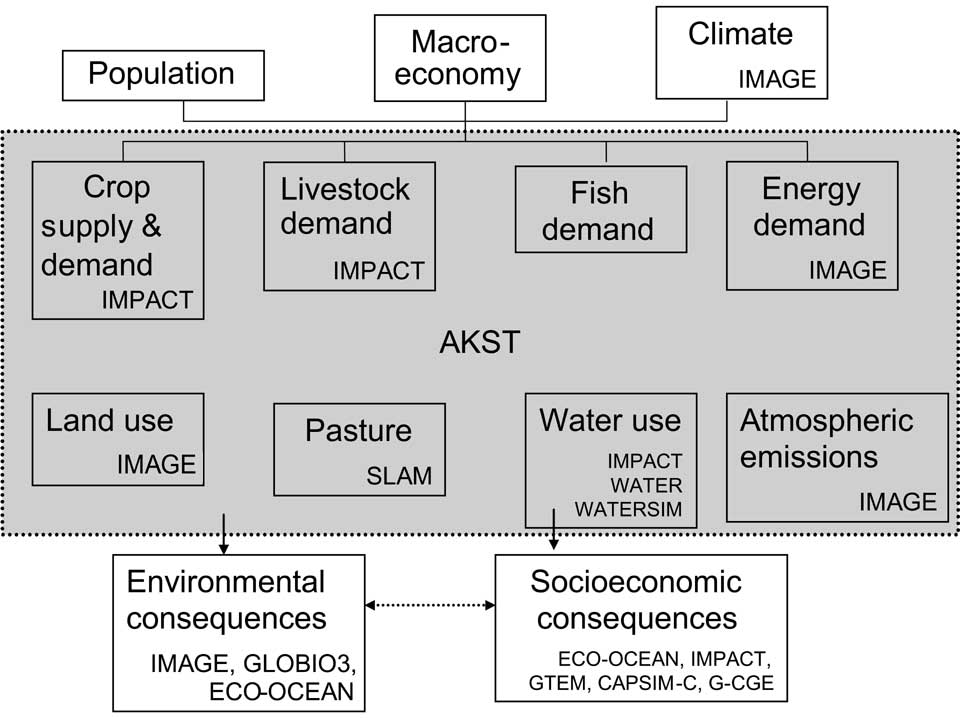
Figure 5-1. Interaction of models in this assessment. Source: Authors.