Outlook on Agricultural Changes and Its Drivers | 285

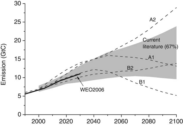
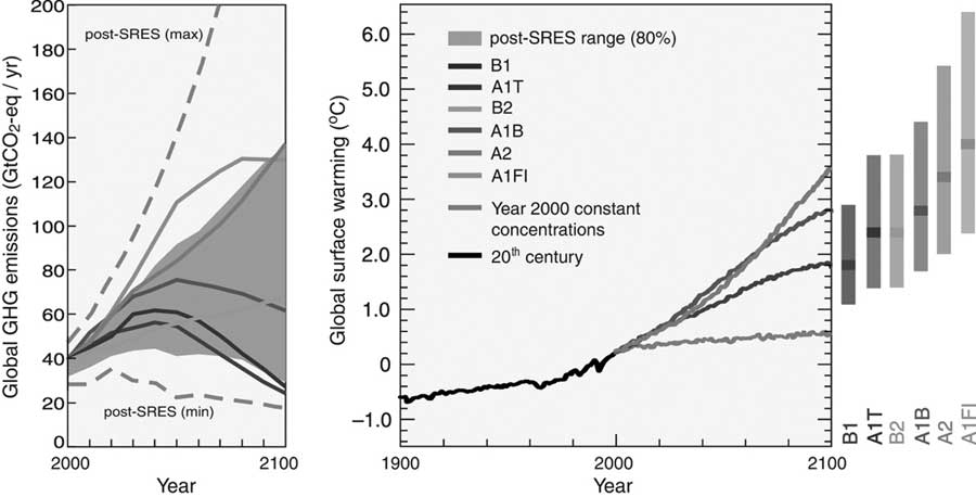
Figure 4-21. Comparison of current CO  emission scenarios (scenarios since IPCC's Third Assessment Report 2001; mean + std. deviation), IPCC-SRES (A1, A2, B1, B2) and WEO2006. sulfur emissions. The latter are currently having a cool­ing effect on the atmosphere. Whereas the computation of global mean temperature is uncertain, the patterns of local temperature change are even more uncertain (Figure 4-24) (IPCC, 2007a).      For precipitation, climate models can currently provide insight into overall global and regional trends but cannot provide accurate estimates of future precipitation patterns in situations where the landscape plays an important role (e.g., mountainous or hilly areas). A typical result of climate

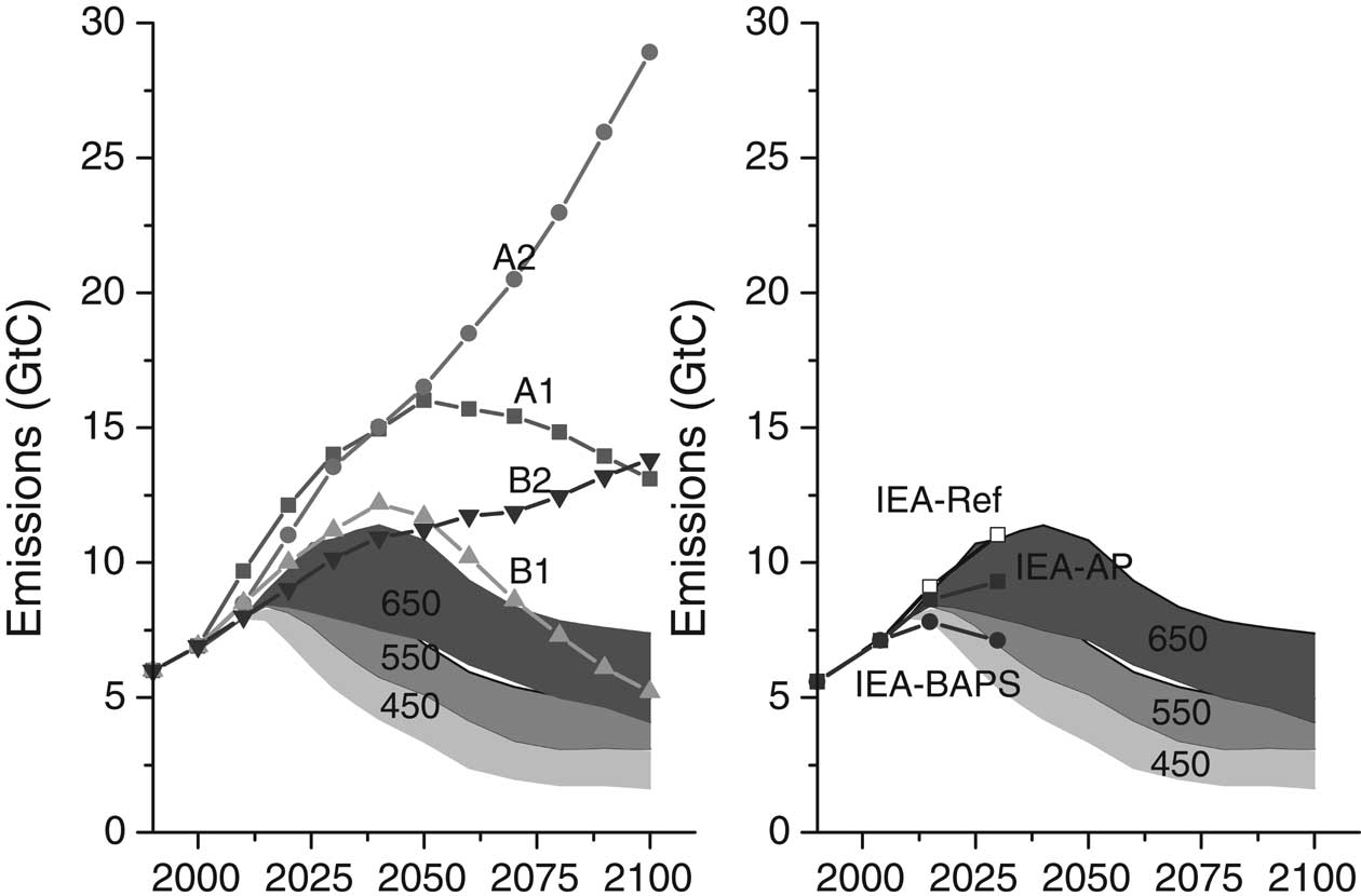
Figure 4-22. Comparison of emission pathways leading to 650, 550 and 450 ppm CO2-eq. and the IPCC-SRES scenarios (left) and the WEO-2006 scenarios. models is that approximately three-quarters of the land sur­face has increasing precipitation. However, some arid areas become even drier, including the Middle East, parts of China, southern Europe, northeast Brazil, and west of the Andes in Latin America. This will increase water stress in these areas. In other areas rainfall increases may be more than offset by increase in evaporation caused by higher temperatures.      Although climate models do not agree on the spatial pat­terns of changes in precipitation, they do agree that global average precipitation will increase over this century. This is

Figure 4-23. Scenarios for GHG emissions from 2000 to 2100 (in the absence of climate policies) and projections of surface temperatures. Source, IPCC, 2007.

Left Panel: Global GHG emissions (in GtCO2-eq) in the absence of climate policies: six illustrative marker scenarios (solid lines) and the 80th percentile range of recent scenarios published since 2000 (shaded area). Dashed lines show the full range of scenarios since 2000. Right Panel: Solid lines are multi-model global averages of surface warming for scenarios A2, A1B and B1, shown as continuations of the 20th-century simulations. The lowest line is not a scenario, but is for Atmosphere-Ocean General Circulation Model (AOGCM) simulations where atmospheric concentrations are held constant at year 2000 values. The bars at the right of the figure indicate the best estimate (solid line within each bar) and the likely range assessed for the marker scenarios at 2090-2099. All temperatures are relative to the period 1980-1999.

Figure 4-23. Scenarios for GHG emissions from 2000 to 2100 (in the absence of climate policies) and projections of surface temperatures. Source, IPCC, 2007.

Left Panel: Global GHG emissions (in GtCO2-eq) in the absence of climate policies: six illustrative marker scenarios (solid lines) and the 80th percentile range of recent scenarios published since 2000 (shaded area). Dashed lines show the full range of scenarios since 2000. Right Panel: Solid lines are multi-model global averages of surface warming for scenarios A2, A1B and B1, shown as continuations of the 20th-century simulations. The lowest line is not a scenario, but is for Atmosphere-Ocean General Circulation Model (AOGCM) simulations where atmospheric concentrations are held constant at year 2000 values. The bars at the right of the figure indicate the best estimate (solid line within each bar) and the likely range assessed for the marker scenarios at 2090-2099. All temperatures are relative to the period 1980-1999.